5.2 Monopolist's Optimal Choice

We are now ready to calculate the monopolist’s optimal choice — that is, to answer the first question posed in the previous section: how much to produce, or, equivalently, what price to choose?

As with any other firm, the monopolist’s optimal choice is determined by the condition that marginal revenue equals marginal cost. The following figure illustrates how to compute the optimal choice in the example discussed earlier: demand curve $P = 5 - Q/1000$ and marginal cost $MC = 2$.

In general, assuming a linear demand curve $P = a - bQ$, and denoting by $c$ the value of the monopolist’s marginal cost (in the example above, $c = 2$), the profit-maximizing condition $MR = MC$ becomes $a - 2bQ = c$, from which we derive the monopolist’s optimal quantity:

\(\begin{gathered} Q = \frac{a - c}{2b} \end{gathered}\)

Substituting this quantity into the demand curve gives the monopoly price:

\(\begin{gathered} P = \frac{a + c}{2} \end{gathered}\)

Comparison with Perfect Competition

The price set by a monopolist is higher than marginal cost, unlike in perfect competition, where in the long run we have

\(\begin{gathered} P = c \quad \text{and} \quad Q = \frac{a - c}{b} \end{gathered}\)

Compared 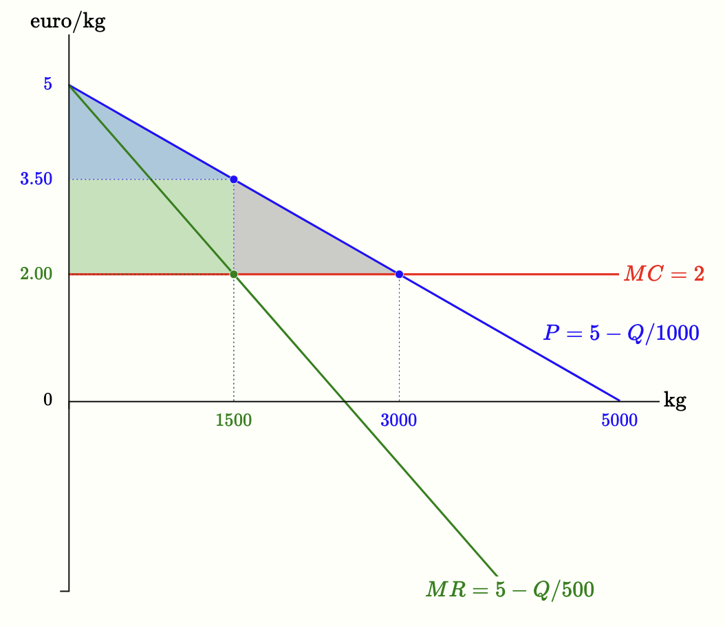to the case of perfect competition, the monopolist therefore produces a smaller quantity (half as much) and charges a higher price. This implies that total surplus is not maximized — there is a monopoly deadweight loss, represented by the grey triangle in Figure 5.5 (reproduced here on the side). In that example, the monopolist produces $1500$ units and charges a price of 3.50 euros. If output were increased, the price would have to be lowered even on units already sold, and profit (the green area) would shrink. For this reason, the quantity produced is below the socially efficient level — the competitive quantity, equal to $3000$ units.

In the introduction we saw an initial illustration of the principle that whenever total surplus in a market is not maximized, one can imagine an alternative allocation that would be unanimously preferred. That is exactly what happens here. How could everyone — monopolist and consumers — be made better off? If output rose from $1500$ to $3000$ units and the price fell from 3.50 to 2.00 euros, consumer surplus would grow by the green area plus the grey area (3375 euros), while the monopolist would lose the green area (2250). But this means that consumers would be willing to “buy” this change from the monopolist at a price higher than the amount for which the monopolist would be willing to “sell” it. By offering the monopolist a transfer between 2250 and 3375, the monopolist would receive more than he loses and consumers would still obtain a net gain.

In practice, consumers do not have a collective organization. There are consumer protection associations such as Altroconsumo in Italy or BEUC at the European level, but they cannot organize collective transfers on this scale. The inefficiency therefore does not arise from a mistake by the monopolist, who rationally maximizes his own profit, but from the fact that such an agreement cannot be carried out. Coordinating millions of consumers so that they all sit at the same table and each contribute their share is simply impossible. It is precisely this lack of coordination on the demand side that makes the agreement impracticable and leaves the deadweight loss of welfare intact.

Monopolist's Markup

One of the most important implications of the monopolist’s behavior concerns the markup, or Lerner index, that is, the difference between price and marginal cost, relative to the price:

\(\begin{gathered} \frac{P - MC}{P} \end{gathered}\)

It is in fact easy to see that the monopolist’s markup is equal to the inverse (with a negative sign) of the price elasticity of demand:

\(\begin{gathered} \frac{P - MC}{P} = -\frac{1}{E^D} \end{gathered}\)

where $E^D$ is the elasticity of demand at the profit-maximizing choice. Indeed, at the optimum we have $MR=MC$, and we also know that $MR=P(1+1/E^D)$. From these two facts the result follows immediately.

Two properties follow from this relationship. First, the monopolist always chooses a point where demand is elastic. If this were not the case (that is, if the firm were on an inelastic segment), an increase in price would raise total revenue and reduce costs, thereby increasing profit: such a point could not be optimal. In fact, from the Lerner formula it follows that, if $MC > 0$, then $ | E^D | > 1$.

Second, The Lerner index can be used to measure a firm’s market power even without knowing its costs. If the price elasticity of demand can be estimated empirically, it is possible to infer the markup the firm is applying. the markup is higher (and thus the price is higher) the less elastic the demand is at the optimum point. In other words, if the absolute value of elasticity is low, the ratio $(P-MC)/P$ is large and the monopolist can charge a relatively high price; conversely, with high elasticity, the markup is small and the price remains close to marginal cost. This explains why in markets where consumers have few alternatives or cannot easily forgo the purchase, prices tend to be high, while in markets with many close substitutes, competitive pressure keeps prices lower.