6.2 Competition on Quantity
In a 2025 interview, the
 president of the Unione Italiana Vini issued a strong appeal to producers in the sector:
“We can no longer afford harvests of 50 million hectolitres... Producing more does not mean earning more. The consequence? A drop in value, with the average production price falling by double digits.”
The reasoning is clear: if each producer decides to increase their output, the market price of wine — which will form only months later, at the time of sale — risks falling for everyone, reducing profit margins. At the same time, the call to “not produce too much” reflects the hope that other producers will behave similarly, limiting overall supply to support prices.
This concrete situation illustrates three key aspects of strategic interaction among firms in many markets. First, in contexts where production takes time or cannot be easily adjusted, quantity is chosen in advance and is therefore the strategic variable — decided before the price forms. Second, each firm is aware that its decisions affect the market price: there is strategic interdependence. Third, there is a tension between individual and collective interest: competition leads to greater production (and thus lower total profit) compared to monopoly.
In the previous
 In 1838 Antoine Augustin Cournot was the first to describe duopoly mathematically as competition in quantities. He also gave the first mathematical analysis of monopoly, which we examined in the first two sections of Chapter 5.
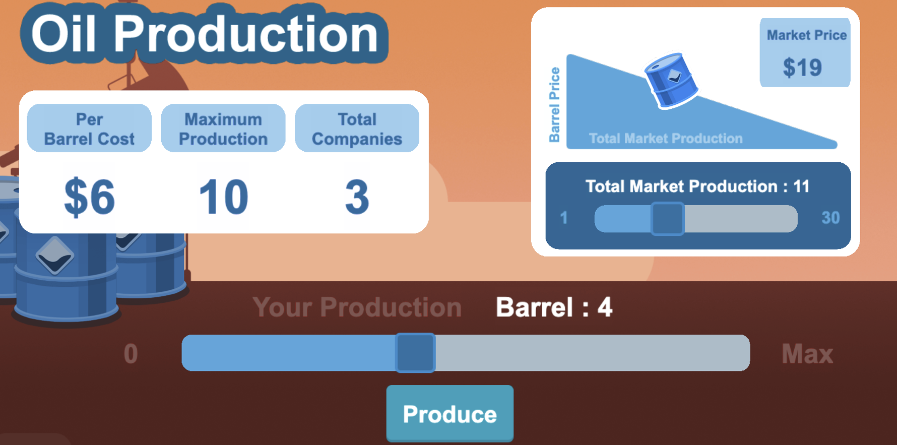
chapter, we examined this kind of strategic interaction through a simplified duopoly model, in which each firm could choose only from a limited number of production levels. In this section, we introduce the Cournot duopoly, which extends that analysis by allowing each firm to choose any non-negative quantity. Firms choose their quantities simultaneously, and the price forms afterward, so that total supply matches demand. The model describes markets where oligopolistic firms must set their output before the price forms — for example, because production requires long lead times. A classic example is the crude oil market, where major producers (such as OPEC countries) decide
In the case of wine, the model’s adherence to reality is more limited, as the market is fragmented across many small producers.
in advance how much to extract and refine, knowing that the price will be determined later based on aggregate supply and global demand.
In 1838 Antoine Augustin Cournot was the first to describe duopoly mathematically as competition in quantities. He also gave the first mathematical analysis of monopoly, which we examined in the first two sections of Chapter 5.
chapter, we examined this kind of strategic interaction through a simplified duopoly model, in which each firm could choose only from a limited number of production levels. In this section, we introduce the Cournot duopoly, which extends that analysis by allowing each firm to choose any non-negative quantity. Firms choose their quantities simultaneously, and the price forms afterward, so that total supply matches demand. The model describes markets where oligopolistic firms must set their output before the price forms — for example, because production requires long lead times. A classic example is the crude oil market, where major producers (such as OPEC countries) decide
In the case of wine, the model’s adherence to reality is more limited, as the market is fragmented across many small producers.
in advance how much to extract and refine, knowing that the price will be determined later based on aggregate supply and global demand.
Before analyzing the full Cournot model, however, we will consider another simplified version — this time assuming a richer set of strategies for each firm. This will help us better understand the equilibrium in the more general game where any non-negative quantity is allowed.
Show firm 1’s best reply Show firm 2’s best reply
| 1600 | 2240 | 0 | 1920 | 240 | 1600 | 400 | 1280 | 480 | 960 | 480 | 640 | 400 | 320 | 240 | 0 | 0 | -320 | -320 | |
| 1400 | 2240 | 0 | 1960 | 280 | 1680 | 480 | 1400 | 600 | 1120 | 640 | 840 | 600 | 560 | 480 | 280 | 280 | 0 | 0 | |
| 1200 | 2160 | 0 | 1920 | 320 | 1680 | 560 | 1440 | 720 | 1200 | 800 | 960 | 800 | 720 | 720 | 480 | 560 | 240 | 320 | |
| 1000 | 2000 | 0 | 1800 | 360 | 1600 | 640 | 1400 | 840 | 1200 | 960 | 1000 | 1000 | 800 | 960 | 600 | 840 | 400 | 640 | |
| $\text{Firm 1}$ | 800 | 1760 | 0 | 1600 | 400 | 1440 | 720 | 1280 | 960 | 1120 | 1120 | 960 | 1200 | 800 | 1200 | 640 | 1120 | 480 | 960 |
| 600 | 1440 | 0 | 1320 | 440 | 1200 | 800 | 1080 | 1080 | 960 | 1280 | 840 | 1400 | 720 | 1440 | 600 | 1400 | 480 | 1280 | |
| 400 | 1040 | 0 | 960 | 480 | 880 | 880 | 800 | 1200 | 720 | 1440 | 640 | 1600 | 560 | 1680 | 480 | 1680 | 400 | 1600 | |
| 200 | 560 | 0 | 520 | 520 | 480 | 960 | 440 | 1320 | 400 | 1600 | 360 | 1800 | 320 | 1920 | 280 | 1960 | 240 | 1920 | |
| 0 | 0 | 0 | 0 | 560 | 0 | 1040 | 0 | 1440 | 0 | 1760 | 0 | 2000 | 0 | 2160 | 0 | 2240 | 0 | 2240 | |
| 0 | 200 | 400 | 600 | 800 | 1000 | 1200 | 1400 | 1600 | |||||||||||
| $\text{Firm 2}$ | |||||||||||||||||||
If we imagine the game matrix shown above as a Cartesian plane, we can think of the possible strategy profiles (the cells of the matrix) as points on that plane, and the strategies of firms 1 and 2 as the corresponding vertical and horizontal coordinates. This is precisely how we represent the Cournot duopoly. Firm 1 chooses a quantity (a point on the vertical axis), firm 2 chooses another (a point on the horizontal axis), and market demand determines the price and hence the corresponding payoffs (profits).
The following figure illustrates the computation of best responses and the Cournot-Nash equilibrium. In the graph, it is possible to manipulate the parameters of the demand curve, which we assume to be linear in the form $P = a - bQ$, and the marginal cost $MC = c$, constant and identical for both firms.
As one would naturally expect, the equilibrium quantity increases if demand is higher — that is, if $a$ increases or $b$ decreases — or if the marginal cost $c$ decreases. Recalling that $c=AC_\text{min}$, since each firm operates at the efficient scale of production in its units, a reduction in $c$ may reflect a technological improvement, or a decrease in fixed costs or wages. The equilibrium is symmetric: the firms produce the same quantity. This depends on the fact that we assumed they have the same marginal cost. It is easy to see, by repeating the calculation of the best responses, that if instead the marginal costs were different, in equilibrium the firm with the lower cost would produce a larger quantity.
Comparison among Market Structures
The Cournot model allows for a clear comparison of equilibrium outcomes across different market structures. With linear demand $P = a - bQ$ and constant marginal cost $MC = AC_\text{min} = c $, we saw in Chapter 5 that a monopolist chooses a quantity equal to half of what would be produced under perfect competition. In this same section, we found that with two firms competing à la Cournot, the total quantity produced is two-thirds of the competitive level. More generally, it can be easily shown that with $n$ firms competing à la Cournot, the total equilibrium quantity equals a fraction $n/(n+1)$ of the competitive quantity — as the number of firms increases, the market outcome gradually converges to that of perfect competition. The following table summarizes these results.
| Market structure | Total quantity | Market price |
|---|---|---|
| Monopoly | \( \dfrac{a - c}{2b} \) | \( \dfrac{a + c}{2} \) |
| Cournot duopoly | \( \dfrac{2(a - c)}{3b} \) | \( \dfrac{a + 2c}{3} \) |
| Cournot with $n$ firms | \( \dfrac{n(a - c)}{(n + 1)b} \) | \( \dfrac{a + nc}{n + 1} \) |
| Perfect competition | \( \dfrac{a - c}{b} \) | \( c \) |
The table shows how the equilibrium outcome depends on the market structure. As the number of firms increases, total quantity approaches the level of perfect competition, and the price falls toward the marginal cost. Producer surplus declines, but consumer surplus grows more rapidly, so that total surplus increases overall. Even with more firms, the Cournot model reveals a tension between individual and collective interest: each firm has an incentive to produce more to increase its own profit, but if all firms behave this way, the price falls and profits shrink for everyone. The result is an intermediate outcome, in which the quantity produced is higher than under monopoly but lower than under perfect competition.